Title
Predicting GPS TEC Maps Using Deep Spatio-Temporal Residual Networks
Contents
- GSoC 2018 Project
- Abstract
- Broad Steps
- People
- Infrastructure
- Phase 1
- Timeline 1: May 14 to May 28
- Exploring GPS TEC Maps and OMNI IMF data
- Plotting TEC Maps
- Specifications of ST-ResNet architecture
- Timeline 2: May 29 to June 11
- Input Data Pipeline
- Generating Input Data Points
- Implementing ST-ResNet Architecture in Tensorflow
- Timeline 3: June 12 to June 17
- Input batch generation
- Tuning ST-ResNet model and Plotting of Results
- Timeline 1: May 14 to May 28
- Phase 2
- Timeline 4: June 18 to June 26
- Getting the difference and channel wise TEC map plots
- Error plots based on difference plots for further analysis
- Timeline 5: June 27 to July 4
- OMNI IMF data preprocessing
- Implementing GRU encoder module
- Results comparison with and without exogenous module
- Timeline 6: July 5 to July 9
- Modifying the code for predicting the next one hour (block) TEC maps
- Reporting the results on block prediction
- Timeline 4: June 18 to June 26
- Phase 3
- Timeline 7: July 10 to July 17
- Implementing the data pipeline in OOPs manner
- Utils files for batch creation during training and testing
- Code testing
- Timeline 8: July 18 to July 28
- Dask implementation for lazy loading of data
- IMF data normalization
- Model training on larger TEC data
- Timeline 9: July 29 to August 8
- Model training based on various hyperparameter values
- Prediction scripts
- Loss and learning curve plots
- Timeline 10: August 9 to August 14
- Final code cleaning and documentation
- Timeline 7: July 10 to July 17
- Final Results
- Future Work
- References
Abstract
Global Positioning System obtained Total Electron Content (GPS TEC) Map is an important descriptive quantity of the ionosphere for analysis of space weather. Building an accurate predictive model for TEC maps can help in anticipating adverse ionospheric effects (ex: due to a solar storm), thereby safeguarding critical communication, energy and navigation infrastructure. In this work, we employ a deep learning approach to predict TEC maps using deep Spatio-Temporal Residual Networks (ST-ResNets), the first attempted work of its kind, by focusing on the North American region. To obtain a contextual awareness of other space weather indicators during prediction, we also use exogenous data including OMNI IMF data (By, Bz, Vx, Np). Our model predicts TEC maps for the next hour and beyond, at a time resolution of five minutes, providing state-of-the-art prediction accuracy. Towards explainable Artificial Intelligence (AI), especially in deep learning models, we provide extensive visualizations of the outputs from our convolutional networks in all three branches (closeness, period and trend) for better analysis and insight. In the future, we aim to demonstrate the effectiveness and robustness of our model in predicting extremely rare solar storms, a challenging task given the insufficient training data for such events.
Project Outline
| S.No. | Step | Status | Date |
|---|---|---|---|
| Phase 1 | |||
| 1 | Dataset exploration: plotting TEC | DONE | May 14 |
| 2 | Dataset preprocessing: missing values | DONE | May 24 |
| 3 | Input pipeline: closeness, period, trend | DONE | May 28 |
| 4 | Model: ST-ResNet in Tensoflow | DONE | June 2 |
| 5 | Model debugging | DONE | June 12 |
| 6 | Results & plots of output TEC maps | DONE | June 12 |
| Phase 2 | |||
| 7 | Difference and Channel wise TEC map plots | DONE | June 19 |
| 8 | Error plots for analysis | DONE | June 22 |
| 9 | OMNI IMF data preprocessing | DONE | June 27 |
| 10 | GRU encoder module | DONE | June 27 |
| 11 | Improved results with IMF data | DONE | July 4 |
| 12 | Block prediction (next one hour) | DONE | July 9 |
| Phase 3 | |||
| 13 | Modifying data pipeline and implementing utils | DONE | July 14 |
| 14 | Training on larger data | DONE | July 17 |
| 15 | Dask implementation and IMF normalization | DONE | July 20 |
| 16 | Model variants training on larger data | DONE | July 30 |
| 17 | Prediction scripts and Learning curves | DONE | August 8 |
| 18 | Final code cleaning and documentation | DONE | August 13 |
People
- Sneha Singhania (sneha3295[at]gmail[dot]com)
- Bharat Kunduri (bharatr[at]vt[dot]edu)
- Muhammad Rafiq (rafiq[at]vt[dot]edu)
Infrastructure
We have used the HPCC system available at Virginia Tech for training the deep learning models on the entire dataset and Google Colab free GPU for training the model on a very small sample of the dataset. I’m highly thankful to the Space@VT organisation for arranging such a high end resource which was very helpful for training and testing various models.
Phase 1
In the first phase of the project, the TEC maps and IMF data are explored. The deep learning model ST-ResNet is designed and implemented in Tensorflow. The model is also trained on a minimal sample of the dataset and preliminary results are reported.
Timeline 1: May 14 to May 28
- Read about GPS TEC Maps, IMF data and other geomagnetic indices
- Plotting the TEC Maps
- Discussion on the specifications of ST-ResNet Architecture
GPS TEC Maps
TEC is the total number of electrons integrated between two points, along a tube of one meter squared cross section. It is a descriptive quantity for the ionosphere of the Earth atmosphere. It can be used for anticipating adverse ionospheric events like solar storms. For this project, we use GPS TEC Maps provided by the MIT Haystack Observatory (Madrigal database). This data is further pre-processed using techniques like median filtering. The TEC maps in its original form and in pre-processed form using median filtering is available at the SuperDARN database of Virginia Tech. For our project, we focus using the median filtered TEC maps.
The TEC maps are stored in a tablular format in text file format. The major columns present in the data are date & time, magnetic latitude, magnetic longitude, TEC values, degree of magnetic latitude resolution and degree of magnetic longitude resoltion. The TEC values are recorded at a resolution of five minutes. We focus on the North-American sector of the TEC maps whose magnetic latitude lies in the range [15, 89] and magnetic longitude lies in the range [250, 360] and [0, 34]. From each text file, we read the TEC values in the given ranges and store it in separate numpy arrays of shape (75, 73).
We also plot TEC maps using the matplotlib library for better understanding. Visualization of TEC maps helps in understanding the spatial- temporal patterns present and can be used further for designing the specifics of the deep learning model. A sample plot of TEC map is shown in the figure below.
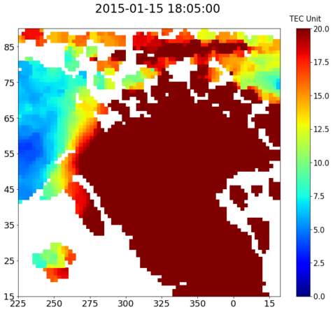 |
|---|
| Figure 1: Sample TEC Plot |
IMF Data
Along with the TEC maps, we use other exogenous data including the OMNI IMF data for better model prediction. The list of exogenous variables that can be used are as follows:
- Bz - OMNI IMF z component
- By - OMNI IMF y component
- Vx - Plasma bulk velocity in km/s along x-axis
- Np - Proton number density
Motivation
The presence of complex spatial and temporal properties in the TEC maps leads us to design deep learning based neural network models. Neural networks form high-dimensional abstract feature representation of the input data and use them for better TEC map predictions. The availability of large scale input TEC maps can be used for obtaining a generalized predictive model. We use the spatial properties of a TEC map and the temporal properties between the TEC maps are used for designing our model called Spatio-Temporal Residual Networks.
ST-ResNet Architecture
Spatio-Temporal Residual Networks (ST-ResNet) is a deep learning model build using Residual Networks. Residual networks (ResNet), variant of Convolutional Neural Networks (CNNs), is a 152 layer network architecture generally used for tasks like classification, detection, and localization of objects. It had won ImageNet Large Scale Visual Recognition Competition (ILSVRC) 2015 challenge and have been used extensively since then. In the deep learning literatute, neural networks suffer from vanishing gradient problem as we keep increasing depth of the model. ResNet overcomes this problem with the help of residual links or skip connections. Deep residual networks helps in creating complex abstract features which leads to better model results.
ST-ResNet consists of three ResNet modules and a Gated Recurrent Unit (GRU) encoder module. The spatial properties of past TEC maps are captured by the convolution operation of the residual network. Further, the temporal properties of past maps are divided into closeness(recent), period(near) and trend(distant), and are captured by three separate residual network branches. As the name suggests, the closeness module takes the input TEC maps present in the recent past (eg. at time resolution of five minutes), period module takes the input TEC maps present at near (eg. at time resolution of one hour) and trend module takes the input TEC maps present at distant (eg. at time resolution of three hour) compared to the future TEC maps to be predicted. The input to the ST-ResNet model is a 3D volume / tensor of past TEC maps stacked behind each other. The output of the three branches are dynamically aggregated with weights learned during training for getting the final accurate prediction.
To obtain a contextual awareness of other space weather indicators during prediction, we integrate exogenous OMNI IMF data (By, Bz, Vx, Np) in an end-to-end fashion, through a Gated Recurrent Unit (GRU) encoder module in our model. GRU helps to process the IMF data in a sequential manner and combine with the ResNet outputs for getting the final prediction. The model architecture is shown in the figure below.
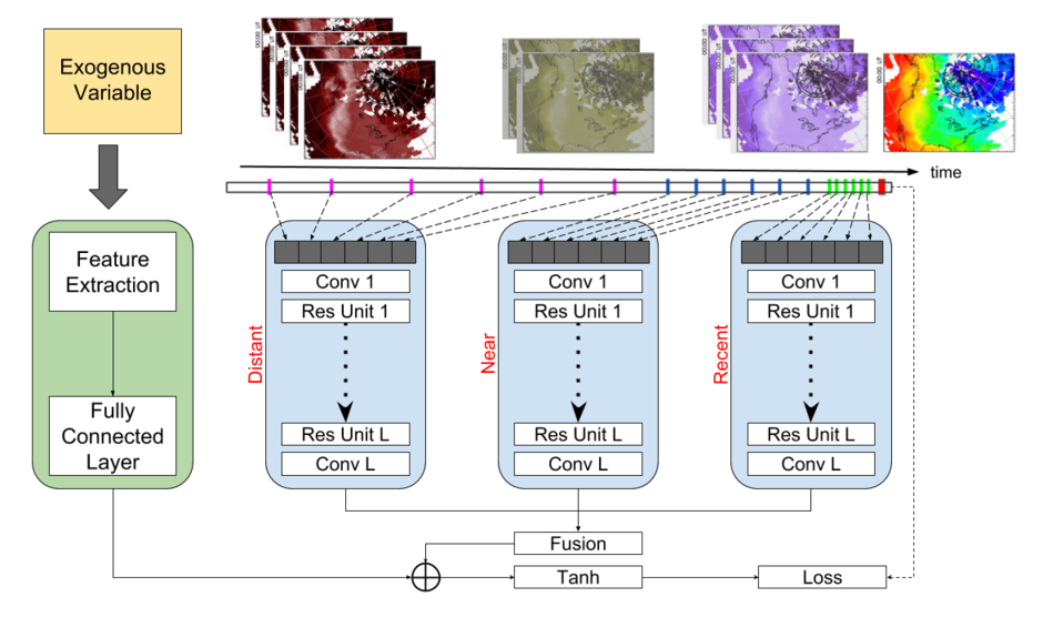 |
|---|
| Figure 2: ST-ResNet Architecture |
Timeline 2: May 29 to June 11
- Setting up input data pipeline
- Creating TEC data points for the model
- Implementing ST-ResNet Architecture in Tensorflow
TEC Data Points
We use the TEC data available in the text files. The TEC values for a particular date and time are extracted and stored as a 2D numpy array. The rows of the array corresponds to the magnetic latitudes and the columns corresponds to the magnetic longitudes. The pandas library is very useful in dealing with tabular data. The TEC data is read into the dataframe and the pivot function is used for selecting the required TEC values in the particular latitude-longitude range. All the TEC maps corresponding to date and time are created and then the sampling algorithm is used for creating the input data points. The number of input TEC maps for each of the ResNet modules are hyperparamters which will be set to accurate values after multiple trainings. As an example, one input data point will contain three different stack of TEC maps of size (12, 75, 73) for closeness module, (24, 75, 73) for period module and (8, 75, 73) for trend module.
Model Implementation
We implement ST-ResNet model in Tensorflow following OOPs paradigm for better modularity. The complex model architecture parts are abstracted through extensive use of functions which brings in more flexibility and helps in coding Tensorflow functionality like sharing of tensors. The four major files which are implemented are main.py, params.py, modules.py and st_resnet.py.
File structure and details:
main.py: This file contains the main program. The computation graph for ST-ResNet is built and launched in a session.params.py: This file contains class Params for hyperparameter declarations.modules.py: This file contain helper functions and custom neural layers. The functions help in abstracting the complexity of the architecture and Tensorflow features. These functions get called for defining the entire computational graph.st_resnet.py: This file defines the Tensorflow computation graph for the ST-ResNet architecture. The skeleton of the architecture from inputs to outputs is defined here using calls to functions defined in modules.py. Modularity ensures that the functioning of a component can be easily modified in modules.py without changing the skeleton of the ST-ResNet architecture defined in this file.
The complete code for the model in Tensorflow is available at the GitHub Repository DeepPredTEC.
Timeline 3: June 12 to June 17
- Input batch generation
- Fine tuning the ST-ResNet model and plotting the results
Given the start time and end time for model training, the TEC data points are loaded into the memory. The TEC data points for training and testing the model is given in batches which is implemented using the yield function of python.
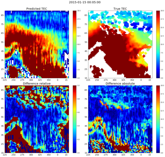
The ST-ResNet model is trained using AdamOptimizer function of Tensorflow. We report preliminary results on predicting the next TEC map by training the model on a small subset of the TEC data. Sample output predicted by the model is shown in the figures below.
Sample with a comparatively lower loss (left figure is the predicted TEC map and the right one is the ground truth):
 |
|---|
| Figure 3: Future TEC Prediction on a Date and Time Near Training Data Points |
Sample with a comparatively higher loss(left figure is the predicted TEC map and the right one is the ground truth):
 |
|---|
| Figure 4: Future TEC Prediction on a Date and Time Farther from Training Data Points |
Presentation
Phase 2
The major focus in the second phase of the project is on getting a better understanding of the model through plotting of intermediate outputs and results. Results are also analysed before and after integration of IMF data processed through GRU network. The models scalability is analysed by predicting the TEC maps for the next one hour at a time resolution of five minutes.
Timeline 4: June 18 to June 26
- Getting the difference and channel wise TEC map plots
- Error plots based on difference plots for further analysis
Difference Plots
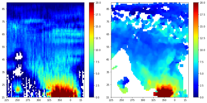
The model was completely implemented in Tensorflow. Without considersing the exogenous module, the model is trained on a fraction of the dataset and the accuracy are reported in a qualitative manner. The predicted maps are plotted and the results are analysed by looking at the absolute and relative difference at each location between the true TEC map and predicted TEC map. The sample predicted plot along with the difference plots is given below.
 |
|---|
| Figure 5: Difference Plot Between the True and Predicted TEC Map Without IMF |
Channel Wise Output Plots
Not only the final output, but the output from each of the ResNet channels, closeness, period and trend, are also plotted for better understanding of the patterns that are being captured by the model. This also helps in evaluating the importance of each of the channels and will further help in model parameter tuning. The sample channel wise output plots for the predicted TEC map is given below.
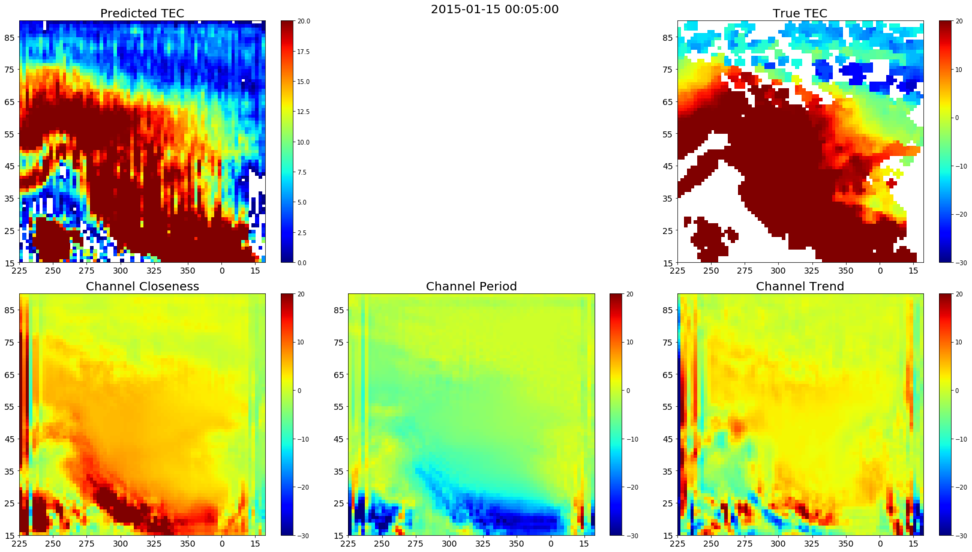 |
|---|
| Figure 6: Channel Wise Plot for a Sample Predicted TEC Map Without IMF |
Timeline 5: June 27 to July 4
- OMNI IMF data preprocessing
- Implementing GRU encoder module
- Results comparison with and without exogenous module
IMF data preprocessing
From the list of exogenous variables, only the IMF data including Bz (OMNI IMF z component), By (OMNI IMF y component), Vx which is the plasma bulk velocity in km/s along x-axis and Np which is the proton number density is taken as an input to the exogenous module. The IMF data is available in a sqlite3 database. Using the forward filling mechanism the missing rows corresponding to the date & time are filled and updated in the original database.
GRU Encoder Module
The IMF data with preprocessing is given as an input to the exogenous module which is based on an GRU architecture. IMF data is loaded with a look back window which is initialized as one of the hyperparamters of the model. GRU takes the (Bz, By, Vx, Np) vectors in a sequential manner based on the date & time associated with it and outputs an abstract complex representation by considering the temporal dependencies present between them.
Improved Results with IMF data
The model is trained by considering the ResNet modules and the exogenous module. The output of the predicted TEC map is analysed with the integration of the IMF data. Results show that IMF data helps in more accurate and smooth prediction at majority of the locations. The sample predicted and difference plot after integration with IMF data is given below.
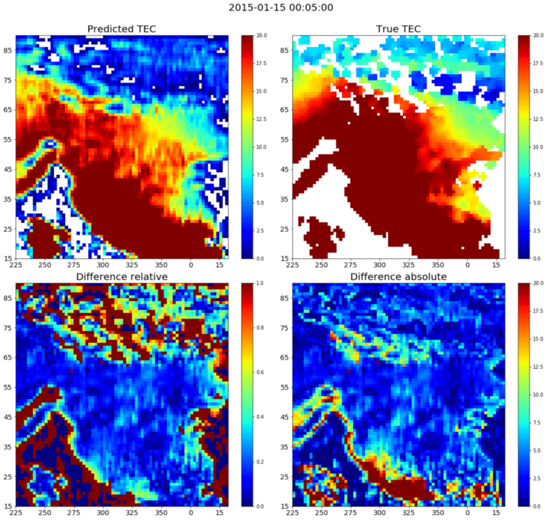 |
|---|
| Figure 5: Difference Plot Between the True and Predicted TEC Map With IMF |
The channel wise output plots with the IMF data integration helps us to understand the change in behaviour of the channels after dynamic integration of channel outputs with the GRU output. It also helps us to understand the relationship between the TEC maps and the IMF data. The sample channel wise output plots with IMF data integration is given below.
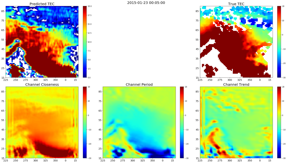 |
|---|
| Figure 6: Channel Wise Plot for a Sample Predicted TEC Map With IMF |
Timeline 6: July 5 to July 9
- Modifying the code for predicting the next one hour (block) TEC maps
- Reporting the results on block prediction
Block prediction (next one hour)
The major aim of using the deep learning model for predicting TEC maps was to obtain a generalized and scalable model. Instead of predicting only the next TEC map, the model now tries solve the harder task of predicting the next one hour TEC maps at a time resolution of five minutes given the past TEC maps as the input. This helps us in understanding the model’s scalability and will further help us in tuning the input TEC maps to each of the channels. On a minimally trained model the accuracy results are reported. The sample block (next one hour) predicted TEC maps are given below.
Presentation
Phase 3
In the phase 3 of the project, the data pipeline is completely written in an object-oriented manner for easy loading of large TEC data. The code is completely tested by checking intermediate output values. We also incorporate dask implementation into the data pipeline for enabling lazy data loading during batch creation. IMF data is normalized and lots of variants of the ST-ResNet model are trained to tune the hyperparameters. We complete the prediction scripts and get the learning curves to understand the model behaviour. Finally we do the code cleaning and document the work done.
Timeline 7: July 10 to July 17
- Implementing the data pipeline in OOPs manner
- Utils files for batch creation during training and testing
- Code testing
Input data pipeline
One of the major challenges of this project is handling the large data input pipeline. The TEC maps are available for about six years from 2011 to 2016 and we would like to train the model on the largerst data size possible. We have implemented the data pipeline using OOPs paradigm with full modularity in Python. The major files implemented are generate_tec_map_files.py, filter_tec_map.py, create_tec_map_table.py and fill_missing_tec_map.py. The functionality of each of these files is explained below.
File structure and details:
generate_tec_map_files.py: This file reads in the median filtered TEC maps from the text file and loads it into a dataframe using the pandas library. It focuses on the North-American magnetic latitudes and longitude ranges and generates a 2D numpy array for each TEC map corresponding to the date & time value present in the text file. The TEC maps are processed by filling the missing TEC values due to missing magnetic latitude or longitude values to get a fixed shape of (75, 73) for all the TEC maps.filter_tec_map.py: This file reads the TEC maps stored in the numpy array and fills the ‘Nan’ or missing TEC values with -1.create_tec_map_table.py: This file creates a new sqlite3 database with filepath and datetime as the fields. For the given start datetime and end datetime range of the TEC maps, it iterates through all the data & time TEC maps from the start datetime and keeps track of the corresponding filepath of filled 2D numpy TEC array. This way we keep track of all the missing TEC maps at a particular datetime.fill_missing_tec_map.py: This file reads the sqlite3 database that was created and gets the date & time of the missing TEC maps and fills it using the nearest date & time TEC map available in the neighbouring window.
Batch and OMNI IMF utils
Once we store the TEC maps in 2D numpy array, we need util files for handling the data points creation and batch creation used at the time of training and testing the deep learning model. The hyperparameters of the ST-ResNet model initialized in params.py are extensively used for creating the TEC data points. The utils files batch_utils.py and omn_utils.py are implemented.
File structure and details:
batch_utils.py: This file contains two major classes calledBatchDateUtilsandTECUtils. TheBatchDateUtilsobject is initialized in themain.pyof ST-ResNet model for creating a dictionary of datetime variables. The key in the dictionary is the current date & time from which the past TEC maps have to be used for data point creation and corresponding value in the dictionary is a numpy array of input datetime variables for the three channels (closeness, period and trend) of the model and the output TEC maps used as the true label during model training. When the Tensorflow session gets initialized for training and testing the model inmain.pythe above mentioned dictionary is used for loading the tensor of actual 2D numpy TEC maps with the help ofTECUtilsclass.omn_utils.py: This file contains theOmnDataclass used for loading the OMNI IMF data originally stored in a sqlite3 database and creating the sequential IMF data array for (By, Bz, Vx, Np) based on a look back window. This look back window is a hyperparameter of the model and can be tuned later. The missing IMF values are filled using forward filling algorithm of pandas library.
Code testing
After implementing the data pipeline and utils functions one of the crucial stages of the project is code testing. We check the input and output values correctness at every step starting from data creation till prediction of TEC map.
Timeline 8: July 18 to July 28
- Dask implementation for lazy loading of data
- IMF data normalization
- Model training on larger TEC data
Dask implementation
As the model complexity is high and input TEC data points are large, the running time for training the ST-ResNet model is quiet high. The HPCC system we use for training the model is a multi-core machine with GPU clusters. Therefore, we modify the actual data loading in the TECUtils class present in batch_utils.py with dask implementation. Dask has Python like APIs and works with the existing Python ecosystem to scale it to multi-core machines and distributed clusters. The dask.delayed function loads the actual TEC maps in a lazy loading manner and has significantly improved the load time of the TEC maps during the training and testing batch creation.
IMF normalization
We normalize each of the OMNI IMF data using z-score. The OMNI IMF data is present in the sqlite3 database with columns corresponding to (By, Bz, Vx, Np). Z-score normalizes each column by substracting the column values with the corresponding column mean and then dividing the column values with the corresponding column standard deviation. This is implemented in the omn_utils.py file.
Model training phase 1
We start our first phase of model training by initializing the hyperparameters with different values. We experiment by changing the batch_size, ResNet depth, number of filters and kernel size used in the convolution layer and GRU hidden size. We train the model and get the predictions for each of them during the same date & time for better output comparison.
Timeline 9: July 29 to August 8
- Model training based on various hyperparameter values
- Prediction scripts and results
- Plotting training loss curve, validation loss curve and bias-variance (learning curve) plots
Model training phase 2
Based on the experiments first phase of model training, we realize that depth of the ResNet plays in important role in getting an accurate prediction. Higher the depth better were the results. We further experiment by running models with different combination of past TEC maps given as an input to each of the channels. We see that closeness channel plays an important role in getting better predictions. We train the model for high number of epochs with a trade off between batch size, resnet depth and input tensors to each of the channels for finding the best model parameters.
Prediction scripts and results
We implement the scripts for getting the predicted TEC maps given the saved trained model as an input. The final predicted TEC map, true TEC map and the channel outputs before final aggregation are stored as numpy arrays for each date & time predicted TEC map.
Plotting training and validation loss curves
The training loss and validation loss values are used for plotting the loss curve for better understanding of the model performance. We plot train and validation loss over the number of epochs to understand when the model overfits on the given data.
Plotting the learning curve
Learning curve helps us to understand the model’s performance given the model complexity and the size of the input data given during training. We train a variant of the ST-ResNet model on varying input data size for training and get the learning curve which is a plot on average training loss vs the input data size for training.
Timeline 10: August 9 to August 14
- Final code cleaning and documentation
Future Work
- Getting better predictions for a longer duration like a day
- Getting the better predictions for rare solar storms events
- Modifying current model architecture using domain knowledge for better results
- Improving the data pipeline further
- Trying out other deep learning based models like Recurrent Neural Networks(RNNs) and Autoencoders